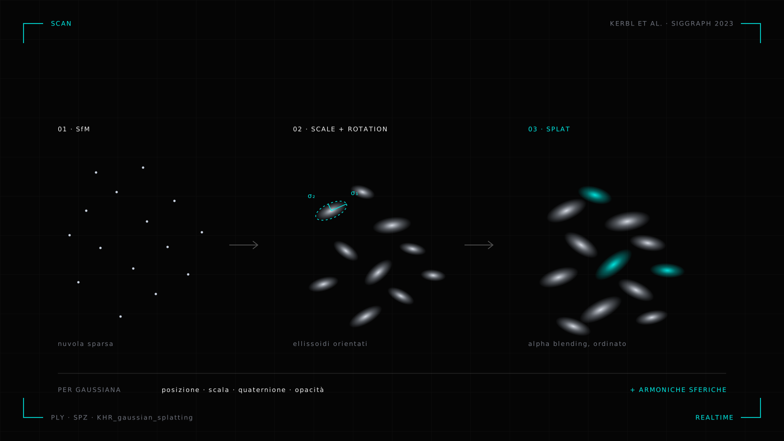
In July 2023 four researchers across Inria and the Max Planck Institute — Bernhard Kerbl, Georgios Kopanas, Thomas Leimkühler and George Drettakis — presented a paper at SIGGRAPH titled 3D Gaussian Splatting for Real-Time Radiance Field Rendering. In three years that technique has gone from academic code to a ratified glTF extension, and it has changed how people talk about 3D capture.
It is worth understanding properly, because it is the kind of technology that gets oversold in both directions: some present it as the end of photogrammetry, others dismiss it as an effect. It is neither.
The problem it solves
Until 2020, reconstructing a scene from photographs meant, in practice, producing a mesh: triangles and textures. Then came NeRFs (Mildenhall et al., 2020), which inverted the approach: instead of building geometry, you train a neural network to answer the question "from this point, looking in this direction, what colour do I see and how dense is the matter?". The visual result is remarkable, because it captures reflections, transparency and volume that a mesh loses.
The problem with NeRFs is cost. The scene lives inside the weights of a network: generating an image means marching rays through the volume and sampling the network dozens of times per pixel. Hours of training, and rendering that in 2020 was nowhere near real time. NVIDIA's Instant-NGP (2022) cut those times dramatically with hash grid structures, but the nature of the computation stayed the same.
Gaussian splatting changes the question. Instead of a continuous function to query, it uses an explicit representation: a set of primitives you can draw with a graphics card the way graphics cards have always drawn things. That is where the performance jump comes from.
What is inside a Gaussian
The scene is a cloud of blurred, overlapping, semi-transparent ellipsoids. Each one is an anisotropic three-dimensional Gaussian, carrying four groups of parameters.
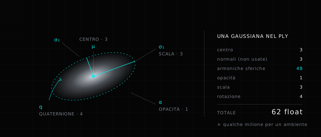
Position. The centre of the ellipsoid, the mean of the distribution: three numbers.
Shape and orientation. The covariance matrix describes how far the Gaussian spreads and in which direction. Optimising it directly does not work, because gradient descent wanders out of the space of valid matrices. So it is factorised into scale (three numbers, the semi-axes) and rotation (a quaternion, four numbers), then recomposed. That is why exchange formats carry separate SCALE and ROTATION rather than six covariance coefficients.
Opacity. How much the Gaussian contributes over whatever sits behind it: one value.
View-dependent colour. This is the NeRF inheritance. Colour is not fixed: it is expressed with spherical harmonics, a basis of functions on the sphere describing how colour changes with viewing direction. Degree zero is the diffuse colour, the same from everywhere; higher degrees add angular variation, and that is how a highlight on a glossy surface travels as you orbit the object. The reference implementation defaults to third degree, which is sixteen coefficients per channel: 48 numbers per Gaussian for colour alone.
Added together, one Gaussian in the PLY file produced by the original implementation takes 62 floating-point values, three of which are normals the method never uses and that sit there for format compatibility. A medium-sized environment settles at a few million Gaussians: the count adds up quickly.
How it is trained
The starting point is classical photogrammetry: images go through a structure from motion pipeline — typically COLMAP — which estimates camera poses and returns a sparse point cloud. Those points become the initial set of Gaussians, initialised small and isotropic.
Then optimisation begins, and this is where the technique is elegant. Rendering is differentiable: you draw the scene from a known camera pose, compare the result with the real photograph, compute the error and propagate it back to the parameters of every Gaussian. Positions, scales, rotations, opacities and harmonic coefficients all adjust together, iteration after iteration.
What makes it work is adaptive densification.
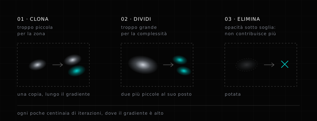
Every few hundred iterations the algorithm looks at where the gradient is large, meaning where the reconstruction is wrong, and acts in two opposite ways. If a Gaussian is too small to cover a region of detail, it clones it. If a Gaussian is large and trying to represent a complex region on its own, it splits it in two. In parallel, Gaussians that have become too transparent are pruned. The cloud grows where detail is needed and thins out where it is not, with nobody deciding the primitive count up front.
Times depend on the scene and the card: minutes for a reconstruction that already reads well, tens of minutes to reach the quality reported in the paper.
Why it runs in real time
Rendering does not cast rays: it projects.
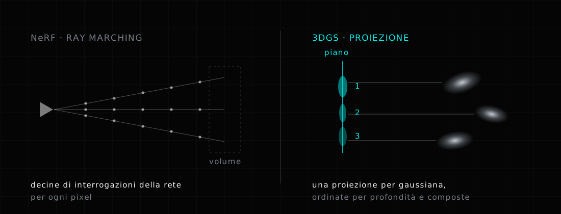
Each three-dimensional Gaussian, seen from a given camera, projects onto the image plane as a two-dimensional Gaussian — a blurred ellipse. This has a long history in graphics, the EWA splatting formalised by Zwicker and colleagues in 2001; the 2023 contribution was making it differentiable and building a rasteriser around it that uses the hardware well.
The rasteriser divides the screen into tiles, assigns each the Gaussians that touch it, sorts them by depth and composites them front to back with alpha blending. Sorting and compositing are things GPUs have done for thirty years.
On the numbers it pays to be precise, because the official sources disagree: Inria's project page claims at least a hundred frames per second at 1080p, while the reference repository is more cautious and states at least thirty. In practice it depends on the scene, the Gaussian count and the card. Either way it is real time, which was the point.
There is a practical consequence that matters more than the performance: Gaussian splatting is a representation, not a trained model. You can inspect it, crop it, merge it, compress it, move it. A NeRF is a black box; a field of Gaussians is a list of objects with coordinates.
Where we stand in 2026
Three years of collective work have produced more variants than are worth listing. Five directions matter.
Geometry. Gaussians are blurred volumes, and extracting a precise surface from them is unnatural. 2D Gaussian Splatting flattens the primitives into oriented discs, which hug surfaces better and give more sensible normals; from there mesh extraction becomes practical. It is the most relevant line of research for anyone who has to work the 3D data afterwards.
Time. 4DGS adds the temporal dimension: Gaussians that move and change over time, which is volumetric video. It is the direction that interests film, sport and performance, and also the one that makes data sizes explode.
Weight. A raw PLY is enormous, and compression has become a field of its own. The SPZ format, released by Niantic under an MIT licence, lands around ten times below the corresponding PLY. It gets there by quantising: positions as 24-bit fixed point, rotations at 10 bits per component keeping only the three smallest of the quaternion and deriving the fourth, scales at 8 bits on a logarithmic scale, colour at 8 bits per channel, and harmonics at five or four bits depending on degree. Every choice is a measured surrender of precision the eye does not catch.
Capture on the move. Several SLAM pipelines build the Gaussian field while the sensor moves, rather than in post. That is the road to real-time capture with handheld devices.
Lighting. In the base model light is baked into the harmonic coefficients: the scene carries the illumination of the day it was photographed and cannot be changed. Separating material from light in order to relight is an open problem, with promising results and no general solution.
The standard has landed
The most concrete news of 2026 is not a paper, it is a format. In February, Khronos announced the release candidate of KHR_gaussian_splatting, a glTF 2.0 extension developed with Autodesk, Cesium/Bentley, Esri, Huawei, Niantic Spatial, NVIDIA and XGRIDS; the extension has since been ratified.
Technically it does something simple and well judged: it uses glTF point primitives and attaches the attributes that matter — ROTATION as a quaternion, SCALE, OPACITY, and the harmonic coefficients, with degree zero required and higher degrees optional. A viewer that has never heard of splats still reads the file as a point cloud instead of rejecting it.
For anyone delivering data to a client this changes a lot. Until recently a splat shipped as a PLY with non-standard attributes, and you hoped the receiving software would interpret it. Now there is a declared container with defined fallback behaviour.
On the software side: Unity has a mature plugin (Aras Pranckevičius', which also reads SPZ), Unreal has several options including those from Volinga and XGRIDS, Cesium brought splats into 3D Tiles with hierarchical levels of detail for large scenes, and web viewers run into the dozens. PlayCanvas' SuperSplat made editing ordinary.
What it cannot do
This is the part usually missing from the presentations.
It is not geometry. A field of Gaussians has no surfaces, no edges, no thickness. You cannot measure a distance across it with the reliability of a laser-scanned point cloud, extract a section, or check a tolerance. Surface-oriented variants improve the situation; they do not reverse it.
The lighting is whatever the weather was. Bringing a splat into an XR scene with its own lighting means, today, accepting that the object carries the shadows of another context.
Reflections and transparency hold up until you get close. Spherical harmonics approximate angular colour variation well, but glass or polished metal seen from positions far from the photographed ones give the game away.
Missing views show. Where there are no photographs, the field invents: Gaussians suspended in mid-air, the so-called floaters. That is fixed by capturing better, not in post.
The weight is real. Even compressed, a quality environment is a serious download for a browser.
Where we use it, and where we do not
Our Scan Lab works with photogrammetry, laser scanners and structured light, and delivers data that has to survive acceptance testing: declared accuracy, verification against independent control points, open formats. In that context Gaussian splatting replaces nothing. Anyone offering you a splat instead of a point cloud to document a heritage site is offering a different thing under the same name.
Where it is the best technique available:
Context and environment for XR experiences. When a real environment has to act as the setting inside an interactive application, a splat delivers it with a fidelity a decimated mesh cannot reach, at a cost that works in real time. This is the case where appearance matters and measurement does not.
Vegetation, complex surfaces, large spaces. Everything that makes traditional photogrammetry produce dirty meshes — leaves, nets, thin objects, environments with a lot of depth — a Gaussian field renders better, because it never has to decide where a surface ends.
Public access. To let someone walk into a place from the browser, as we did for Scurcola Abbey, a splat is in a different class from a lightened model. With the caveat that scientific reconstruction and visual restitution remain two separate deliverables.
Site visits and quick documentation. Half an hour of filming gives you a navigable environment. Not for detailed design: for deciding where to go back and measure.
The sensible way to use it, in our experience, is alongside: laser scanning and photogrammetry give certified geometry, the Gaussian field gives appearance. They are two layers of the same capture, not two alternatives.
What to expect
The two things to watch over the coming months are relighting and surface extraction. If they become reliable, Gaussian splatting stops being a visual layer and becomes a capture format in its own right, with geometry as a by-product. Until then it stays what it is: the most efficient way we know to bring the appearance of a place onto a screen, in real time.
Which is not nothing, considering it did not exist three years ago.
We work on 3D capture and navigable environments: what Scan does, or tell us about your case and we will say which technique makes sense — including using neither.
Sources: Kerbl, Kopanas, Leimkühler, Drettakis, 3D Gaussian Splatting for Real-Time Radiance Field Rendering, SIGGRAPH 2023 · reference implementation, Inria GRAPHDECO · Khronos glTF extension announcement · KHR_gaussian_splatting specification · SPZ format, Niantic